/ THE SHORT ANSWER
- 01Use the authors' neural model before attempting a new whole-brain implementation.
- 02Keep FlyWire and MaleCNS versions, neuron identifiers and files separate.
- 03Download a small circuit rather than the entire microscopy volume.
- 04Treat body physics, neural computation and their interface as separate engineering problems.
- 05Compare your model against controls and real observations, not just an attractive video.
/ dotSuper point of view
Build one experiment you can explain before building a fly you can animate.
A brain map is the beginning, not the executable
It is what we can do with it.
Can you stimulate a circuit, predict which cells respond, change a connection and see what happens?
Yes, with a model.
But downloading the connectome does not download the animal's memories, neural state or behaviour.
A simulation adds mathematical assumptions to structural measurements.
An animated fly adds another layer: a body interacting with an environment.
This guide follows three routes and explains where they meet.
Sources are numbered at the end.
The companion includes setup commands and an original MaleCNS teaching notebook.
We have not executed these tutorials or independently reproduced the papers.
| Your goal | Start here | What you are not getting automatically |
|---|---|---|
| Simulate a neural response to stimulation | Shiu et al.'s FlyWire/Brian2 model | A body, every biological mechanism or a MaleCNS implementation |
| Investigate a circuit in the new male dataset | MaleCNS plus neuprint-python | Measured dynamics or a ready-made controller |
| See a fly-shaped body move in a physics world | flybody and its documented controllers | The original fly's reconstructed brain controlling that movement |
| Study visual motion processing | Flyvis and its pretrained-model tutorials | A general-purpose whole-animal simulation |
First, choose a question small enough to answer
Begin with a measurable change: when I stimulate this input group, does a selected downstream readout respond differently?
For a first neural project, reproduce a sensory-stimulation example from the published model.
For a MaleCNS project, investigate a documented cell type and a bounded set of partners.
For a body project, measure one movement variable under one controller.
Write the hypothesis before choosing the visualization.
Record the input, the readout, the comparison and a result that would contradict your expectation.
This turns a demo into an experiment you can discuss honestly.
A useful first deliverable is a small folder containing the query, model settings, output data, one plot and a paragraph explaining the limitations.
A rotating brain image is optional.
A traceable explanation is not.
FlyWire and MaleCNS are not interchangeable files
This guide targets the documented neuPrint dataset male-cns:v1.0.
The official project provides browser tools and downloadable connectivity resources.
Sources 1 to 3.
The published Shiu model uses FlyWire data from an adult female brain.
Its repository includes a version-630 setup and a separate version-783 file pair.
Replacing one file with a newer download does not constitute a model upgrade.
Source 7.
Keep a dataset manifest.
Include the specimen/resource, release, identifier namespace, filters and download date.
Treat these as part of the model definition, not administrative notes.
A MaleCNS bodyId and a FlyWire root ID identify objects in different resources.
Similar cell-type names can help formulate a comparison, but they are not permission to join tables by number.
| Record | Why it matters |
|---|---|
| Resource and version | Results depend on the reconstruction and annotation release |
| Exact neuron identifiers | Names and annotations can change |
| Included tissue and cell selection | A brain-only model omits much of the motor system |
| Connection threshold and weight definition | Filtering changes the graph before any simulation runs |
| Code revision and dependency environment | A later implementation can produce different behaviour |
Route 1: install the published neural model
The authors provide an environment.yml specifying Python 3.10, Brian2 2.5.1 and NumPy 1.24, along with notebook and data dependencies.
Prefer that starting environment to installing unrelated latest packages into an existing AI project.
Sources 7 and 8.
The commands below follow the repository's installation route.
Run them on your own machine, not inside an already configured notebook kernel.
If Git or Conda is unavailable, install those prerequisites or follow the authors' notebook route.
Open example.ipynb and read the setup cells before running the experiment.
Skip the cell explicitly labelled for Google Colab when running locally.
Keep the supplied neuron and connectivity files together.
Source 9.
Installation is not reproduction.
First establish that the environment loads the selected data.
Then run a deliberately small experiment.
Only after that should you spend time on a complete protocol.
| Step | Command |
|---|---|
| Get the authors' repository | git clone https://github.com/philshiu/Drosophila_brain_model.git |
| Enter the project | cd Drosophila_brain_model |
| Create the supplied environment | conda env create -f environment.yml |
| Activate that environment | conda activate brian2 |
| Open the example notebook | jupyter notebook example.ipynb |
Make the first run small and explicitly provisional
Keep that supplied population for the first experiment rather than choosing a random ID from another connectome.
The output is simulated spike events, not measured activity from a living fly.
Source 9.
Our suggested smoke-run settings are one trial, 100 milliseconds and one worker.
These are editorial scope choices, not the paper's experimental protocol.
Shortening the duration does not avoid loading the underlying network.
In the companion, copy the parameter dictionary before changing it, create a fresh result directory and use a unique experiment name.
This avoids accidentally mixing an exploratory run with previous outputs.
The implementation defaults to skipping an experiment when its output file already exists.
A repeated filename can therefore look like a fresh run when it is not.
Use new names rather than casually enabling overwrite.
Source 10.
Save the exact duration used for each output.
A firing-rate calculation must use that same duration.
Comparing a short exploratory trace with a longer published trial without accounting for timing is not a fair comparison.
Turn one run into a controlled experiment
You might change the input rate, suppress a selected model neuron's influence, or compare two input populations.
Do not change all three at once.
Use a baseline condition and an intervention condition with matching duration and analysis windows.
For stochastic simulations, collect repeated trials and record how random seeds are handled.
A single run cannot establish a robust difference.
Preselect an output population or a physiological readout from the source study.
Selecting the most dramatic responding neuron after every run makes it harder to distinguish a real hypothesis from a convenient story.
Plot the readout over time, the distribution across trials and the difference between conditions.
Report nonresponses too.
An empty or uninformative trace is a debugging clue, not a reason to invent activity.
Finally, compare the intervention with experimental evidence.
A model can be useful even when it fails, provided the failure exposes which assumptions need work.
Agreement in one feeding experiment does not establish fidelity for every behaviour.
- Baseline: the same model and analysis, without the chosen intervention.
- Perturbation: one changed input, connection rule or defined neuron manipulation.
- Sensitivity: repeat with a small, documented change in a modelling parameter.
- Evidence check: identify the biological measurement your output is meant to predict.
- Report: show the uncertainty and describe what would invalidate your interpretation.
Route 2: query a small MaleCNS circuit
DNge104 appears in the download examples, so the companion uses it as a starting seed, not as a claim that it is the right circuit for a particular behaviour.
Sources 2 and 3.
Authenticate to neuPrint using your own account token.
The Python client accepts NEUPRINT_APPLICATION_CREDENTIALS; the notebook alternatively prompts without echoing the token.
Never put credentials in a published notebook, screenshot or shared result file.
Source 4.
Fetch the seed cells, inspect their identifiers and retrieve their direct incoming and outgoing partners.
The companion keeps at most 200 selected neurons and then obtains connections within that selection.
This bounds the retained model, not necessarily the initial server response.
Start by understanding the returned table.
Every connection has a direction.
Keep the presynaptic identifier, postsynaptic identifier and connection weight together.
Do not turn a directed graph into an undirected graph just because the plotting library makes that easier.
Export the graph you intended to export
Its directed connection records avoid the extra aggregation needed when working with per-region adjacency outputs.
Overlapping anatomical regions are not independent bins you can blindly sum.
Source 5.
Preserve raw weights before normalizing anything.
Save the selected neuron list, final edge table and a manifest alongside the model.
Record the threshold even when it seems unimportant.
Selecting only strong neighbours creates a deliberately incomplete circuit.
It can remove weak paths, feedback through excluded cells and relevant sensory input.
The selection is useful for learning the pipeline, not an anatomical boundary.
Do not join labels, neurotransmitter predictions and graph edges until you have checked their release and identifier fields.
Keep identifiers as integers or strings, not floating-point values.
This becomes especially important when handling long FlyWire IDs in spreadsheets or JavaScript.
What the downloadable notebook actually simulates
This makes the data-to-model pipeline inspectable without pretending we have calibrated the circuit's physiology.
Its matrix uses rows for receiving cells and columns for sending cells.
It normalizes incoming positive weights, applies a short input pulse and iterates a leaky, saturating update.
The output is in arbitrary activity units and iteration steps, not hertz or biological milliseconds.
All retained links are treated as positive in this teaching example.
It does not infer excitation, inhibition, neurotransmitter action or consciousness.
Use the published Brian2 route for a biologically motivated neural model instead.
The notebook compares intact propagation with a model-only ablation of a selected non-input node.
It keeps the original normalization after ablation, so the intervention does not silently strengthen the remaining connections.
These plots are generated only when a reader runs the notebook.
We have not inserted fabricated traces or labelled research images as simulation results.
| Output | Interpretation |
|---|---|
| neurons.csv and edges.csv | The selected, versioned structural subgraph |
| manifest.json | Query, selection, package versions, model assumptions and chosen intervention |
| activity.csv | Per-node toy-model activity in arbitrary units |
| activity-comparison.png | A visualization of intact versus ablated toy propagation |
| No output bundled | The notebook is supplied unexecuted, without claimed results |
How to move from a graph toy to a neural model
Choose a neuron model, specify units and time integration, define the input process and document how a recorded connection count becomes a model weight.
Neurotransmitter labels are useful evidence, not a complete synaptic mechanism.
A biologically defensible model also needs an explicit treatment of receptor effects, uncertain classifications and the behaviours it aims to explain.
Keep unknown values visible.
A table labelled 'assumed delay' is more useful than a precise-looking number presented as measured.
Distinguish source measurements, inferred labels, literature parameters and parameters you fitted.
Before fitting to a result, reserve observations for evaluation.
Otherwise you risk demonstrating only that a model can reproduce the data used to tune it.
If you change dataset, do not assume a parameter that worked previously remains appropriate.
Treat the transfer as a new modelling experiment with its own controls.
Route 3: build the body simulation separately
Its published work includes learned controllers for walking and flight.
That is a different contribution from reconstructing the MaleCNS wiring diagram.
Sources 11 and 12.
For a first local setup, the companion uses a separate Python 3.10 environment and the core package installation.
Keep optional training dependencies out until the body and a basic environment load.
The official getting-started notebook also has a Colab route.
Its setup expects a GPU runtime and configures EGL rendering.
Do not paste that GPU-specific configuration unchanged into a local Mac setup.
Source 13.
First inspect the body, load the documented example and render a frame.
Then introduce an actuator command.
A frame establishes that rendering works; an arbitrary action establishes only that the interface accepts controls.
Random actuator values are not a walking policy.
To reproduce the reported locomotion, follow the authors' controller, environment and training or inference instructions, including any separately required data and parameters.
| Milestone | What it establishes |
|---|---|
| Model loads | The geometry and physics assets are available |
| A frame renders | The graphics backend works |
| Actuators change the state | The action interface is connected |
| A documented policy completes a task | That controller works in that environment |
| A connectome model predicts behaviour | A much stronger claim requiring additional evidence |
Connecting the neural model to the body is the hard part
After the body moves, new sensory information must return to the neural model.
Without that return path, you have an open-loop animation.
Define each interface before building it.
What observation reaches the model?
Which cells receive it?
How is neural output transformed into joint commands?
At what rate does each part update?
The matrix of anatomical connections does not answer those engineering questions for you.
Nor does the presence of a ventral nerve cord automatically provide a calibrated neuron-to-actuator mapping.
Begin with one constrained task, such as controlling a turn in a simple environment.
Use a conventional controller as a baseline.
Compare tracking error, falls, task success and sensitivity to disturbances.
If a learned adapter supplies most of the control intelligence, say so.
The connectome may be a structural constraint rather than a faithful reconstruction of the animal's controller.
That can still be interesting without calling it a mind upload.
Four real examples, and what to borrow from each
Their differences are more useful than treating every result as proof that an entire fly has been copied into software.
Shiu and colleagues, Nature 2024: a FlyWire-based computational brain model was used to predict sensorimotor responses, with experimental comparisons involving feeding and grooming.
Borrow the strategy of defining a neural intervention and testing a specific readout.
Do not generalize those results to every behaviour.
Source 6.
Lappalainen and colleagues, Nature 2024: connectome-constrained models were optimized for visual motion processing and evaluated against neural response properties.
Borrow the combination of anatomical constraints, a defined computational task and held-out functional evidence.
The model is not a whole-body simulation.
Source 14.
Vaxenburg and colleagues, Nature 2025: an anatomical body model and learned controllers reproduced naturalistic locomotion in simulation.
Borrow the separation between a physical model and the policy controlling it.
The reported controller is not automatically the newly mapped male CNS.
Source 11.
Jin and colleagues, 2026 arXiv preprint: a connectome-shaped graph controller was trained through deep reinforcement learning for simulated locomotion.
This is relevant to embodied AI, but the cited version is a preprint.
Borrow the baseline comparisons, while treating performance claims as the authors' reported results.
Source 17.
A practical alternative: simulate a visual task
Flyvis provides the official implementation associated with the 2024 visual-system paper.
Its tutorials cover connectome exploration, flash and moving-edge responses, training and custom stimuli.
Sources 15 and 16.
Start with a documented pretrained example before training your own model.
Present a standard stimulus, save the response and explain what was held constant.
Next, change one property of the stimulus, such as its direction, contrast or speed.
Compare the response to a defined expected pattern.
This is more interpretable than showing an arbitrary image and searching for a compelling story afterward.
A good portfolio project explains both the response it predicted and the conditions under which the model stopped being useful.
Where these methods could become useful
Some are established research uses.
Others are engineering hypotheses that need their own evidence.
For neuroscience, a model can prioritize circuit interventions for laboratory testing.
The useful output is a ranked, testable hypothesis, not a claim that computation replaces experiments.
For robotics, a connectome-inspired controller can be compared with a conventional controller under identical training budgets and tasks.
Measure whether the structural constraint improves learning or robustness rather than assuming biological inspiration must be better.
For machine vision, a motion-processing model provides an interpretable setting for studying sensitivity to visual inputs.
Any transfer to an industrial camera system needs separate evaluation on that system's images, latency and failure conditions.
For education, the combination of a real graph, a transparent model and a documented negative result can teach more than a polished simulation video.
For manufacturers and other businesses, these projects are currently more relevant as research methods than as ready-made factory products.
A credible proposal should identify the operational problem before introducing a fly-brain analogy.
Can you start without paid compute?
This is our budget-conscious starting recommendation, not a measured minimum specification.
No paid account or hosted training job is required by the supplied teaching notebook.
The full neural model has a different memory footprint from a 200-node teaching graph.
Reducing its run duration does not shrink the full connectivity representation.
Parallel workers can also increase memory pressure.
Body rendering, policy inference and reinforcement-learning training have different requirements.
Do not assume that successfully rendering one image means your machine can reproduce a training run.
Use free notebook services only within whatever resources they currently provide.
This guide does not promise a free GPU, uninterrupted sessions or a fixed runtime.
Avoid starting paid instances simply because an example offers a cloud deployment option.
Record actual memory use and elapsed time when you run your own experiment.
A useful cost estimate comes from a representative run, not an unsupported promise that every laptop can simulate a fly.
Download connectivity first, not the entire microscope volume
The annotations are smaller.
A targeted neuPrint query avoids starting with those bulk files.
Source 3.
Choose the representation your question requires.
A connectivity experiment needs neuron and edge information.
A geometry project may need skeletons or meshes.
A reconstruction audit may need the underlying images.
Keep coordinate conventions with spatial files.
Combining a mesh, skeleton and external template without checking units can create a plausible-looking but incorrect overlay.
Do not calculate required RAM from a compressed download size alone.
Loading tables, constructing indices and creating simulation objects can add overhead.
Leave room for outputs and keep copies of large data only when they serve a clear purpose.
Make the experiment reproducible before making it impressive
Store a manifest, input hashes, model settings and a short interpretation with the outputs.
Use a fresh directory rather than overwriting yesterday's result.
Separate data preparation from simulation.
Someone should be able to inspect the final neuron and edge tables without needing your notebook's hidden execution history.
Keep the software environment record, but review it before sharing.
Package-version lists are useful; dumped environment variables can leak credentials.
The supplied notebook records a small whitelist of package versions instead.
Caption every image honestly.
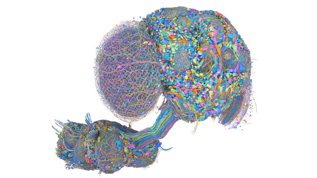
The hero on this article is an attributed Janelia research rendering.
It is not a result from our notebook, a recording of neural activity or a demonstration that our code ran.
Report the model's scope in the first sentence of any public claim.
'A toy propagation model on a selected MaleCNS subgraph' and 'a biologically validated whole-animal simulation' are not interchangeable descriptions.
- Dataset identity, release, selection criteria and original source.
- Exact neuron identifiers, edge direction and weight transformation.
- Model equations, units, input encoding and intervention.
- Random seeds, trial count and analysis interval where applicable.
- Software versions, source revision and checksums for saved inputs.
- Baseline, comparison metric, uncertainty and known failure conditions.
Common problems and what to inspect first
Authentication, data selection, dynamics and rendering fail for different reasons.
Reinstalling everything at once usually destroys the evidence you need.
| Symptom | First thing to inspect |
|---|---|
| Authentication failure | Your own neuPrint login/token and the requested dataset, without sharing the token |
| The selected type returns no cells | The exact type label and dataset version in the official browser |
| No retained edges | The selected cell set and minimum connection weight |
| A neuron ID is missing | Identifier namespace and the matching connectivity/neuron file pair |
| A repeated run produces no new file | Experiment name and the implementation's existing-output behaviour |
| The neural model produces no useful response | Input selection, units, duration and whether the readout belongs to the model |
| Memory use is too high | Graph scope and worker count before increasing paid resources |
| The body loads but rendering fails | Platform-specific graphics backend rather than the connectome |
| The body moves but does not walk | Controller and task configuration, not just action-vector shape |
Questions people ask before their first simulation
You can access structural datasets and supporting resources.
Those downloads are not the animal's complete physiological state, experience or an executable consciousness.
Can I create my own simulation?
Yes.
You can begin with an existing model or create a smaller one with explicit assumptions.
The strength of any biological claim depends on its validation, not the number of neurons included.
Does MaleCNS work directly inside the published FlyWire model?
Not as a drop-in file replacement.
You would need to adapt identifiers, data preparation, model assumptions and evaluation for the new resource.
Can I make it walk?
A physics model and controller can produce movement.
Demonstrating that the reconstructed biological circuit explains that movement is a separate, harder objective.
Do I need to train an AI model?
Not for every project.
Structural queries and a fixed neural simulation are different from learning a control policy.
Choose the method that matches your question.
Is the dataset free to reuse?
The MaleCNS project specifies CC BY 4.0 for its dataset.
Retain attribution and check separate terms for software and media.
A free dataset does not guarantee free computation or institutional endorsement.
Source 1.
A realistic first project to build this week
For neural modelling, reproduce the authors' starting experiment and document one careful manipulation.
For MaleCNS, run the bounded notebook and explain why its graph model is not physiology.
For embodiment, get a documented body environment working before designing a neural controller.
For vision, change one stimulus in a published tutorial and compare the predicted response.
Finish with one page: what you asked, what you used, what changed, what the evidence supports and what remains unknown.
Include enough material for another person to repeat your choices.
The goal is not to claim that you uploaded a fly.
It is to make one useful piece of the connectome-to-simulation pipeline understandable, inspectable and worth building on.
What this page cannot conclude
- 01This guide and its original companion notebook were prepared with AI assistance from the linked primary sources. dotSuper has not executed the tutorial code or independently reproduced the cited studies.
- 02The supplied MaleCNS notebook is a bounded, all-positive teaching model in arbitrary units. It is not a calibrated neural simulation, a whole-animal controller or a scientific reproduction.
- 03Upstream software, authentication, dataset annotations and free compute availability can change. Use the authors' current documentation for operational updates.
- 04Published results and the explicitly labelled arXiv preprint are different evidence levels. Proposed business and robotics applications require their own evaluation.
- 05Research institutions and authors have not endorsed dotSuper or this guide.
Sources
- 011. MaleCNS project and research imageryHHMI Janelia / FlyEM · accessed Sep 15, 2026
- 022. Explore the MaleCNS connectomeMaleCNS project · accessed Sep 15, 2026
- 033. MaleCNS downloads and dataset documentationMaleCNS project · accessed Sep 15, 2026
- 044. neuprint-python authentication and quick startneuPrint developers · accessed Sep 15, 2026
- 055. neuprint-python connectivity query referenceneuPrint developers · accessed Sep 15, 2026
- 066. A Drosophila computational brain model reveals sensorimotor processingShiu and colleagues / Nature, 2024 · accessed Sep 15, 2026
- 077. Published FlyWire brain model: repository and installationShiu and collaborators · accessed Sep 15, 2026
- 088. Published model: Python and Brian2 environmentShiu and collaborators · accessed Sep 15, 2026
- 099. Published model: example experiment notebookShiu and collaborators · accessed Sep 15, 2026
- 1010. Published model: simulation implementationShiu and collaborators · accessed Sep 15, 2026
- 1111. Whole-body physics simulation of fruit fly locomotionVaxenburg and colleagues / Nature, 2025 · accessed Sep 15, 2026
- 1212. flybody: installation, environments and controllersTuraga Lab / HHMI Janelia and Google DeepMind · accessed Sep 15, 2026
- 1313. flybody: official getting-started notebookTuraga Lab · accessed Sep 15, 2026
- 1414. Connectome-constrained networks predict neural activity across the fly visual systemLappalainen and colleagues / Nature, 2024 · accessed Sep 15, 2026
- 1515. Flyvis: official implementation and tutorialsTuraga Lab and collaborators · accessed Sep 15, 2026
- 1616. Flyvis documentation and custom-stimulus tutorialsFlyvis developers · accessed Sep 15, 2026
- 1717. Whole-Brain Connectomic Graph Model Enables Whole-Body Locomotion Control in Fruit FlyJin and colleagues / arXiv preprint, version 3, June 2026 · accessed Sep 15, 2026
- 1818. dotSuper practical companion: commands, code and limitationsdotSuper, original educational material, not executed · accessed Sep 15, 2026
- 1919. What Is a Connectome, and What Is Missing?dotSuper research collection · accessed Sep 15, 2026
- 2020. Can a Fly Brain Run on a Computer?dotSuper research collection · accessed Sep 15, 2026
Our editorial standard · Found an error? Send a correction with its source.
/ CITE OR SHARE THIS GUIDE
Make the evidence easy to verify.
When you reference this guide, link to its canonical URL. That gives readers one stable place for the evidence, limitations and future updates.
dotSuper Research Desk. (September 15, 2026). Build Your First Fruit Fly Brain Simulation. dotSuper. https://dotsuper.net/feeds/applied-systems/how-to-build-fruit-fly-brain-simulation
Explore a MaleCNS Circuit in Jupyter
An unexecuted, annotated notebook for querying a small graph, saving its provenance and comparing toy activity propagation. Full neural-model and flybody setup commands are linked in source 18.
Download the teaching notebook