/ THE SHORT ANSWER
See the method. Keep the context.
The visual companion
Reuse: Original artwork created for dotSuper. No public reuse licence has been specified. Attribution to research sources does not grant rights to their artwork or datasets.
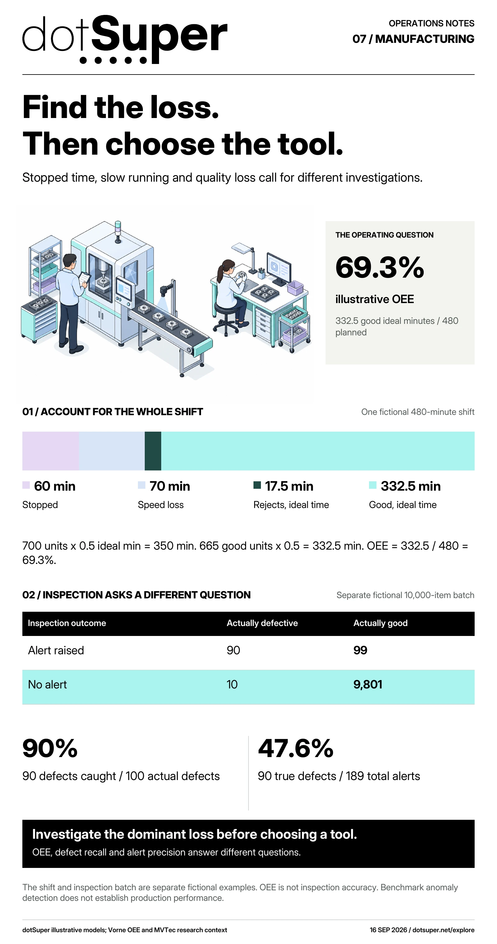
Read the diagram: Stopped time, slow running and quality loss call for different investigations. The shift and inspection batch are separate fictional examples. OEE is not inspection accuracy. Benchmark anomaly detection does not establish production performance.
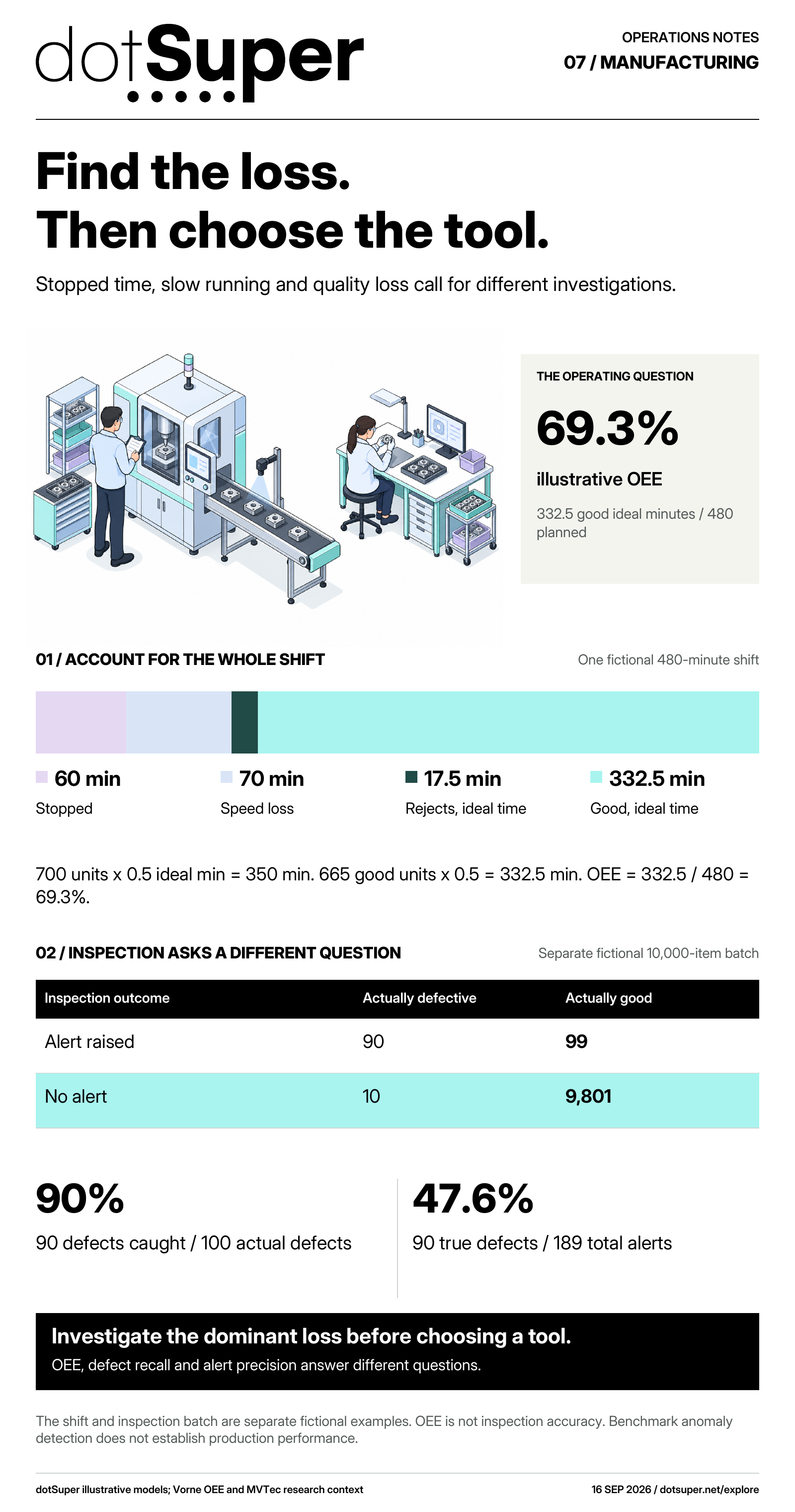
A fictional 480-minute production shift loses 60 minutes to stops, 70 to speed and 17.5 equivalent minutes to rejects, leaving 332.5 ideal minutes of good output and 69.3% OEE. In a separate 10,000-item inspection example, 90 true alerts and 99 false alerts yield 47.6% precision with 90% defect recall.
Fictional shift: 480 planned minutes; 60 stopped; 420 running; 700 total units at 0.5 ideal minutes; 665 first-pass good units. Speed loss is 70 minutes and reject ideal-time loss is 17.5 minutes. Good-output ideal time is 332.5 minutes.
Availability: 420/480 = 87.5%. Performance: 350/420 = 83.3%. Quality: 665/700 = 95%. OEE: 332.5/480 = 69.3%.
Separate inspection batch: 10,000 items, 100 defective; 90 true alerts, ten missed defects, 99 false alerts and 9,801 correct passes. Recall is 90/100 = 90%; precision is 90/189 = 47.6%.
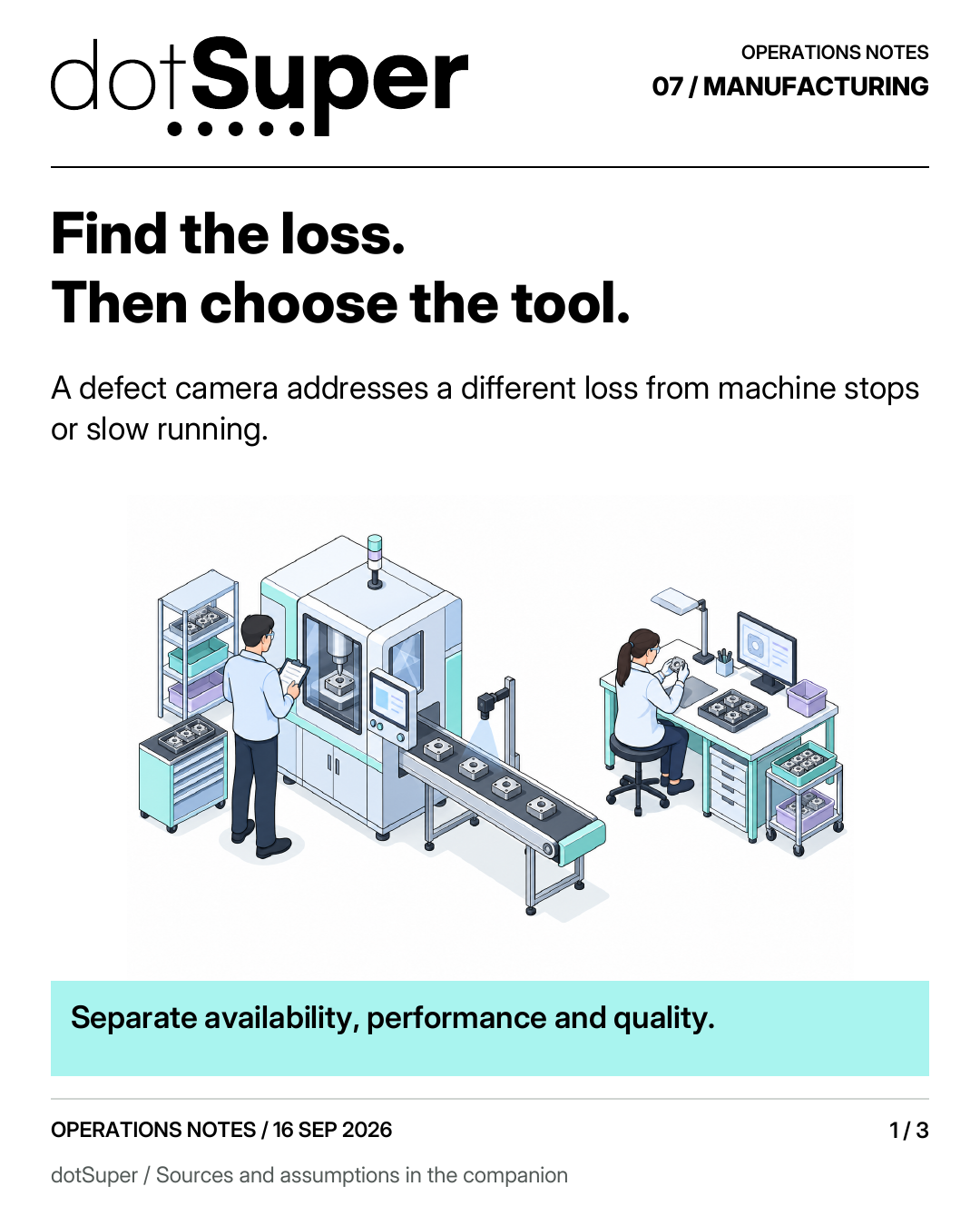
Find the loss. Then choose the tool. A defect camera addresses a different loss from machine stops or slow running. Separate availability, performance and quality.
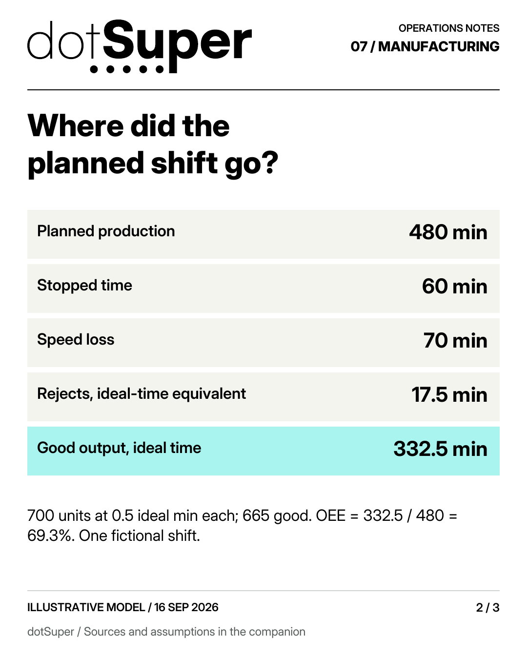
Where did the planned shift go? Planned production / 480 min Stopped time / 60 min Speed loss / 70 min Rejects, ideal-time equivalent / 17.5 min Good output, ideal time / 332.5 min 700 units at 0.5 ideal min each; 665 good. OEE = 332.5 / 480 = 69.3%. One fictional shift.
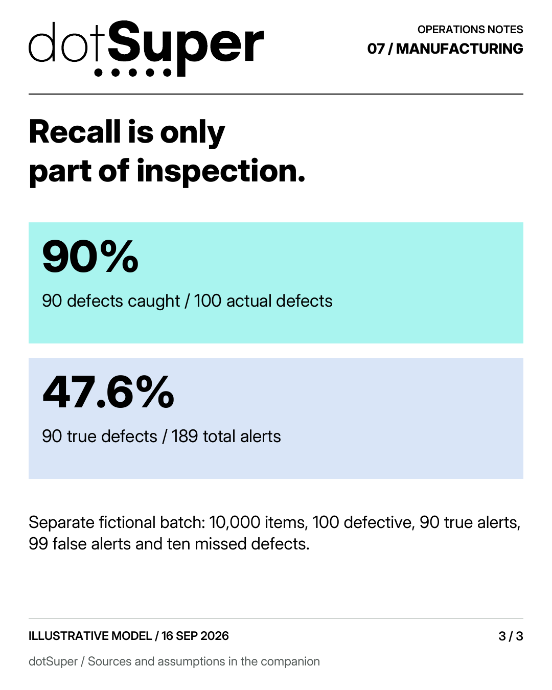
Recall is only part of inspection. 90% / 90 defects caught / 100 actual defects 47.6% / 90 true defects / 189 total alerts Separate fictional batch: 10,000 items, 100 defective, 90 true alerts, 99 false alerts and ten missed defects.
The shift and inspection batch are separate fictional examples. OEE is not detection accuracy.
No local defect rate, downtime-reduction benchmark or universal OEE target is asserted.
MVTec AD is a research benchmark with noncommercial reuse restrictions. No benchmark imagery is reproduced in the original artwork.
This operating explanation does not prescribe autonomous machine-control changes or replace plant engineering procedures.
| Dataset | Observation | Values and conditions |
|---|---|---|
| Fictional example: shift accounting | Planned production | Value: 480; Unit: minutes |
| Fictional example: shift accounting | Stops | Value: 60; Unit: minutes |
| Fictional example: shift accounting | Running | Value: 420; Unit: minutes |
| Fictional example: shift accounting | Ideal time for total output | Value: 350; Unit: minutes |
| Fictional example: shift accounting | Speed loss | Value: 70; Unit: minutes |
| Fictional example: shift accounting | Ideal time for good output | Value: 332.5; Unit: minutes |
| Fictional example: shift accounting | Total produced | Value: 700; Unit: units |
| Fictional example: shift accounting | First-pass good | Value: 665; Unit: units |
| Fictional example: shift accounting | Ideal cycle | Value: 0.5; Unit: minutes per unit |
| Fictional example: shift accounting | Rejects, ideal-time equivalent | Value: 17.5; Unit: minutes |
| Fictional example: shift accounting | Availability | Value: 87.5%; Unit: 420 / 480 |
| Fictional example: shift accounting | Performance | Value: 83.3%; Unit: 350 / 420 |
| Fictional example: shift accounting | Quality | Value: 95%; Unit: 665 / 700 |
| Fictional example: shift accounting | OEE | Value: 69.3%; Unit: 332.5 / 480 |
| Fictional example: inspection confusion matrix | Defective | Flagged: 90; Passed: 10 |
| Fictional example: inspection confusion matrix | Good | Flagged: 99; Passed: 9,801 |
Reuse: Original artwork created for dotSuper. No public reuse licence has been specified. Attribution to research sources does not grant rights to their artwork or datasets.
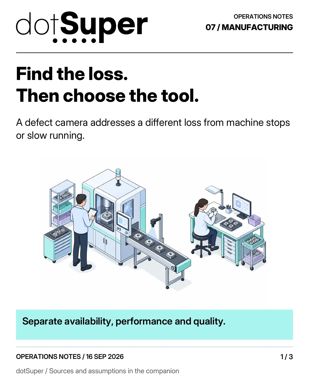
Read the diagram: Panel 1 of 3. Find the loss.
Find the loss. Then choose the tool. A defect camera addresses a different loss from machine stops or slow running. Separate availability, performance and quality.
The shift and inspection batch are separate fictional examples. OEE is not detection accuracy.
Reuse: Original artwork created for dotSuper. No public reuse licence has been specified. Attribution to research sources does not grant rights to their artwork or datasets.
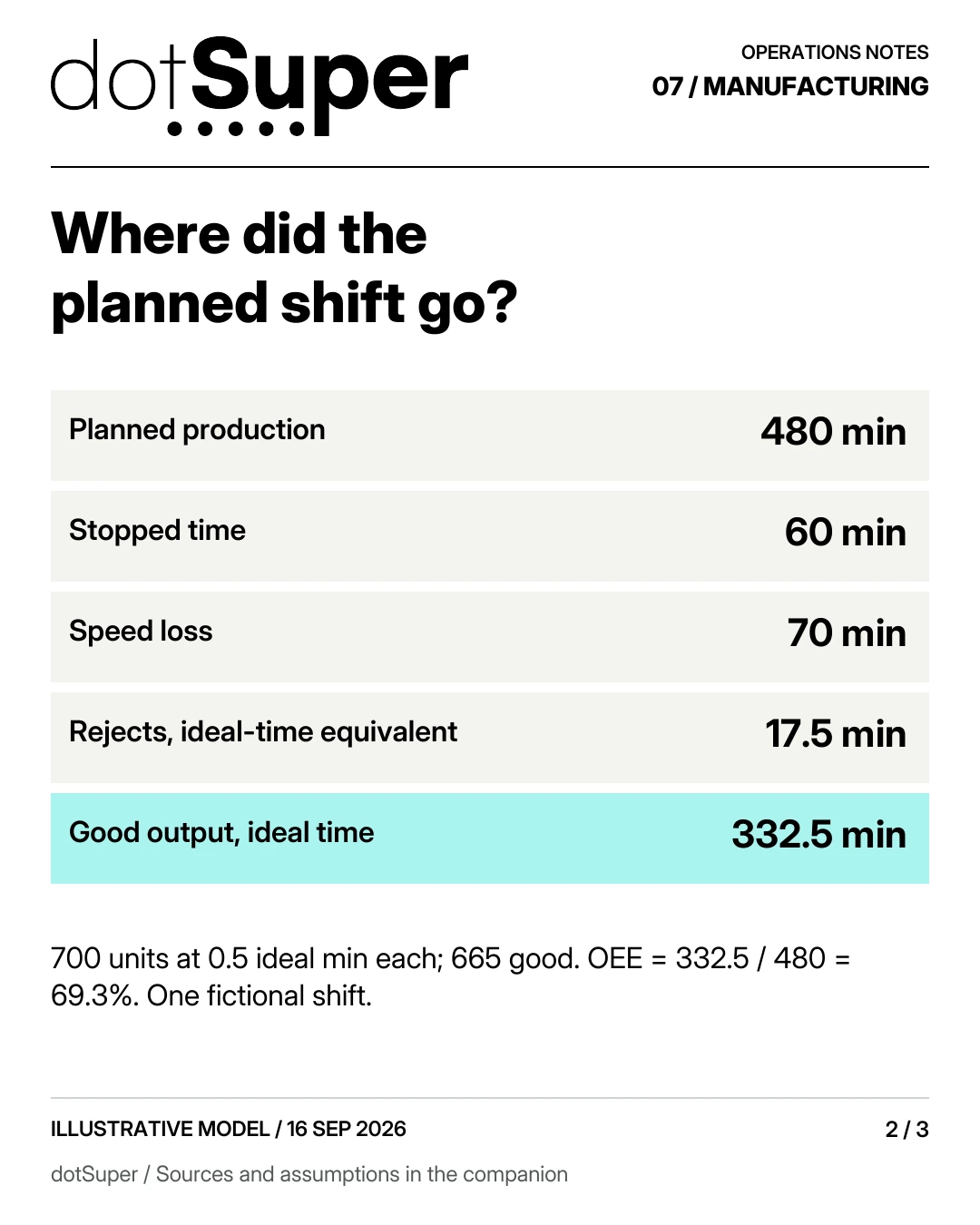
Read the diagram: Panel 2 of 3. Where did the planned shift go? Planned production / 480 min Stopped time / 60 min Speed loss / 70 min Rejects, ideal-time equivalent / 17.5 min Good output, ideal time / 332.5 min 700 units at 0.5 ideal min each; 665 good.
Where did the planned shift go? Planned production / 480 min Stopped time / 60 min Speed loss / 70 min Rejects, ideal-time equivalent / 17.5 min Good output, ideal time / 332.5 min 700 units at 0.5 ideal min each; 665 good. OEE = 332.5 / 480 = 69.3%. One fictional shift.
The shift and inspection batch are separate fictional examples. OEE is not detection accuracy.
Fictional example: shift accounting.
Quantity: Planned production; Value: 480; Unit: minutes.
Quantity: Stops; Value: 60; Unit: minutes.
Quantity: Running; Value: 420; Unit: minutes.
Quantity: Ideal time for total output; Value: 350; Unit: minutes.
Quantity: Speed loss; Value: 70; Unit: minutes.
Quantity: Ideal time for good output; Value: 332.5; Unit: minutes.
Quantity: Total produced; Value: 700; Unit: units.
Quantity: First-pass good; Value: 665; Unit: units.
Quantity: Ideal cycle; Value: 0.5; Unit: minutes per unit.
Quantity: Rejects, ideal-time equivalent; Value: 17.5; Unit: minutes.
Quantity: Availability; Value: 87.5%; Unit: 420 / 480.
Quantity: Performance; Value: 83.3%; Unit: 350 / 420.
Quantity: Quality; Value: 95%; Unit: 665 / 700.
Quantity: OEE; Value: 69.3%; Unit: 332.5 / 480.
| Quantity | Value | Unit |
|---|---|---|
| Planned production | 480 | minutes |
| Stops | 60 | minutes |
| Running | 420 | minutes |
| Ideal time for total output | 350 | minutes |
| Speed loss | 70 | minutes |
| Ideal time for good output | 332.5 | minutes |
| Total produced | 700 | units |
| First-pass good | 665 | units |
| Ideal cycle | 0.5 | minutes per unit |
| Rejects, ideal-time equivalent | 17.5 | minutes |
| Availability | 87.5% | 420 / 480 |
| Performance | 83.3% | 350 / 420 |
| Quality | 95% | 665 / 700 |
| OEE | 69.3% | 332.5 / 480 |
Reuse: Original artwork created for dotSuper. No public reuse licence has been specified. Attribution to research sources does not grant rights to their artwork or datasets.
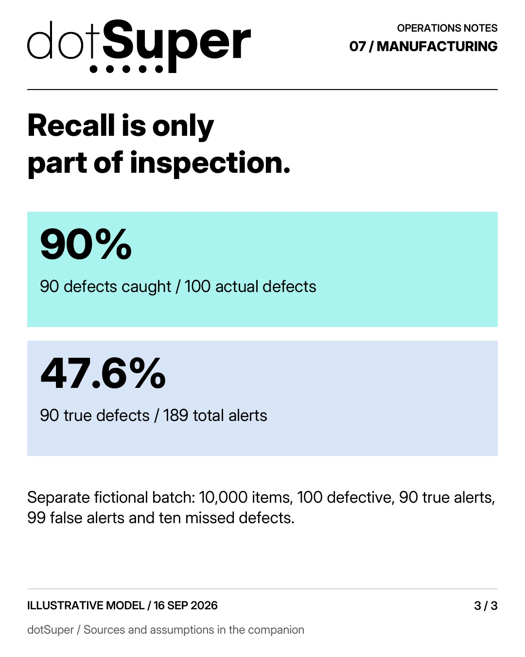
Read the diagram: Panel 3 of 3. Recall is only part of inspection.
Recall is only part of inspection. 90% / 90 defects caught / 100 actual defects 47.6% / 90 true defects / 189 total alerts Separate fictional batch: 10,000 items, 100 defective, 90 true alerts, 99 false alerts and ten missed defects.
The shift and inspection batch are separate fictional examples. OEE is not detection accuracy.
Fictional example: inspection confusion matrix.
Actual class: Defective; Flagged: 90; Passed: 10.
Actual class: Good; Flagged: 99; Passed: 9,801.
| Actual class | Flagged | Passed |
|---|---|---|
| Defective | 90 | 10 |
| Good | 99 | 9,801 |
Take it into your next working session
Keep the source credits with the file. Check the reuse terms and adapt the method to your context.
Credit: dotSuper original fictional worked-example data.
Reuse: Original illustrative data. No public reuse licence has been specified. These are not client measurements or research results.
Credit: dotSuper original fictional worked-example data.
Reuse: Original illustrative data. No public reuse licence has been specified. These are not client measurements or research results.
Reuse: Original artwork created for dotSuper. No public reuse licence has been specified. Attribution to research sources does not grant rights to their artwork or datasets.
Reuse: Original artwork created for dotSuper. No public reuse licence has been specified. Attribution to research sources does not grant rights to their artwork or datasets.
Reuse: Original artwork created for dotSuper. No public reuse licence has been specified. Attribution to research sources does not grant rights to their artwork or datasets.
Reuse: Original artwork created for dotSuper. No public reuse licence has been specified. Attribution to research sources does not grant rights to their artwork or datasets.
Reuse: Original artwork created for dotSuper. No public reuse licence has been specified. Attribution to research sources does not grant rights to their artwork or datasets.
Reuse: Original artwork created for dotSuper. No public reuse licence has been specified. Attribution to research sources does not grant rights to their artwork or datasets.
Thumbnail credit and reuse
Reuse: Original artwork created for dotSuper. No public reuse licence has been specified. Attribution to research sources does not grant rights to their artwork or datasets.
- 01Stopped time, speed loss and quality loss are different quantities and should not be double-counted.
- 02The fictional shift has 332.5 ideal good-output minutes over 480 planned minutes, or 69.3% OEE.
- 03In the separate inspection batch, 90% recall produces only 47.6% precision because false alerts matter.
- 04Evaluate the action after an alert, with actual production prevalence and a practical baseline.
/ dotSuper point of view
Production accounting identifies the loss worth addressing. Inspection recall and precision then describe a particular detection task, not the performance of the whole factory.
Audience, question and answer
Start with a consistent loss definition and the decision that follows detection.
A camera that finds anomalies does not diagnose every quality issue.
A model that predicts a failure is only useful if maintenance can act in time.
Separate inspection, diagnosis, maintenance planning and machine control.
The explanation uses globally relevant manufacturing methods and fictional plant arithmetic.
It makes no Saudi or UAE defect-rate claim.
A local implementation must account for the line, materials, suppliers, working conditions and available maintenance resources.
Evidence and what it does not prove
It is a documented benchmark for industrial visual anomaly detection.
It does not represent a production plant's defect prevalence or the full range of hidden material and process faults.
Bergmann et al., MVTec AD, CVPR 2019 paper (source 1).
The dataset owner states that MVTec AD uses a Creative Commons Attribution-NonCommercial-ShareAlike licence.
A public download does not grant unrestricted commercial reuse; the infographic uses original artwork and reproduces no benchmark images.
MVTec, dataset page, checked 16 September 2026 (source 2).
Vorne's OEE educational material defines the product of availability, performance and quality, and explains the underlying time and output measures.
This is a supplier-authored description of a widely used operating method, not neutral evidence that a particular target is optimal for every plant.
Vorne, OEE calculation, live page checked 16 September 2026 (source 3).
Those sources support a distinction between measuring losses and evaluating one detection method.
They do not establish a universal AI return, a typical downtime reduction or a “world-class” threshold appropriate to every operation.
Avoid importing such percentages from vendor sales material without a documented denominator and comparable context.
Diagnose the loss before selecting the system
Let operators record “unknown” rather than force a guess.
Distinguish a stoppage caused by equipment failure from one caused by missing material or downstream congestion.
The machine being stopped is not necessarily the machine causing the constraint.
For quality, distinguish first-pass defects, rework, scrap and customer escapes.
Count units consistently.
A part repaired and accepted later should not silently become first-pass good output.
Link defect classification to product revision, lot and inspection method.
For downtime, ask what actionable warning exists.
A bearing temperature signal may support condition monitoring; a material shortage may require inventory discipline; a changeover delay may need better standard work.
These interventions have different data and ownership requirements.
A language model summarising maintenance notes is a different project from predictive maintenance based on sensor data.
Map the response to every alert: inspect, adjust, stop, replace, schedule or escalate.
State who decides and how long the response takes.
An alert that arrives five minutes before failure is not useful if spare parts require three days, although it may still support a safe shutdown where properly engineered.
AI assistance must remain within the approved operating boundary.
This explanation does not recommend autonomous machine-control changes.
Safety and process control require qualified engineering review and the plant's applicable procedures.
Worked example: one fictional production shift
The line stops for 60 minutes and runs for 420.
It produces 700 units at an agreed ideal cycle time of 0.5 minutes each, with 665 first-pass good units.
These numbers are illustrative, not an observed factory.
Availability is 420/480 = 87.5%.
Performance is (0.5 × 700)/420 = 83.3%.
Quality is 665/700 = 95%.
OEE is their product, approximately 69.3%.
The equivalent direct calculation is (0.5 × 665)/480 = 69.3%.
The 60 stopped minutes are visible, but the running-period speed loss also matters: the 700 units account for only 350 ideal minutes out of 420 actual run minutes.
That 70-minute gap needs investigation.
Installing a defect camera addresses a different loss from either stopped time or slow running.
If a future test prevents ten defective units at the same total production count, good output rises from 665 to 675.
Quality becomes 96.4% and OEE approximately 70.3%, a gain of about one percentage point.
This is conditional arithmetic, not a forecast.
It does not establish additional sales, lower labour expense or the best investment.
A second example: rare defects and false alarms
A detector catches 90 defects and misses ten.
If it also flags 1% of the 9,900 good items, it produces 99 false alerts.
Of 189 total alerts, only 90 are genuine defects, giving precision of about 47.6% despite 90% defect recall.
This demonstrates why a headline “90% detection” is incomplete.
The quality team must handle 189 alerts, and ten defects still escape detection.
Changing the alert threshold trades one type of error against another.
Select thresholds using the cost and consequence of errors, not just a visually impressive score.
The assumed 1% defect prevalence and false-positive rate are fictional.
Real prevalence can shift by product, lot and season.
A balanced benchmark test set can substantially overstate production precision if its positive share is much higher than the plant's.
Evaluation protocol and quantitative context
Include new lighting, camera movement, dirt, packaging and legitimate product changes.
Record rejected or uninspectable images.
A model should not quietly count unreadable items as good.
For maintenance, evaluate warnings at an action-relevant horizon and count false alarms per asset-time.
Use chronological validation to avoid information from after a failure leaking into predictions.
Record planned interventions that prevented a failure, because the observed outcome is affected by maintenance action.
Compare performance against a practical baseline: current inspection, a simple threshold or existing preventive maintenance.
Measure inspection effort, alert response, missed faults and line disruption.
An offline score is evidence about the dataset, not proof of operating benefit.
Financial evaluation should distinguish avoided scrap, recovered throughput and reduced downtime.
If recovered output cannot be sold or used, do not value it automatically at full sales price.
Avoid counting the same recovered unit in both throughput and scrap benefits.
Evidence and boundaries
Each source supports only the scope stated beside the claim.
| Claim | Source or calculation | Limit |
|---|---|---|
| MVTec AD has 5,354 images and 15 categories | Bergmann et al. 2019 | Benchmark composition, not plant population |
| Dataset has a noncommercial reuse restriction | MVTec dataset page | Check separate permission before commercial imagery |
| OEE combines availability, performance and quality | Vorne calculation guide | Denominator policy must be consistent |
| Example OEE is 69.3% | 332.5 ideal good minutes / 480 planned minutes | Fictional shift |
| Example alert precision is 47.6% | 90 / (90 + 99) | Fictional prevalence and error rates |
| First project should follow the actionable loss | dotSuper analysis | Recommendation to test, not empirical ranking |
One practical next step
Identify the loss and its owner before choosing an inspection, maintenance or workflow intervention.
Counterevidence and limitations
Better classifiers do not establish root cause.
A model may detect a stain while missing an internal material fault.
A plant with inconsistent downtime coding may benefit more from a reliable log and daily review than a prediction model.
OEE can also be gamed by changing planned time or ideal cycle assumptions.
Product mixes and asset roles differ.
Use consistent definitions within a relevant process before comparing plants or countries.
The target should follow customer and operating needs, not a generic league table.
What this page cannot conclude
- 01The shift and inspection batch are separate fictional examples. OEE is not detection accuracy.
- 02No local defect rate, downtime-reduction benchmark or universal OEE target is asserted.
- 03MVTec AD is a research benchmark with noncommercial reuse restrictions. No benchmark imagery is reproduced in the original artwork.
- 04This operating explanation does not prescribe autonomous machine-control changes or replace plant engineering procedures.
Sources
- 01Bergmann et al., MVTec AD, CVPR 2019 paperBergmann and co-authors; CVPR · accessed Sep 16, 2026
- 02MVTec, dataset page, checked 16 September 2026MVTec · accessed Sep 16, 2026
- 03Vorne, OEE calculation, live page checked 16 September 2026Vorne Industries / OEE.com · accessed Sep 16, 2026
Our editorial standard · Found an error? Send a correction with its source.
/ CITE OR SHARE THIS GUIDE
Make the evidence easy to verify.
When you reference this guide, link to its canonical URL. That gives readers one stable place for the evidence, limitations and future updates.
dotSuper Research Desk. (September 17, 2026). Find the loss. Then choose the tool.. dotSuper. https://dotsuper.net/feeds/applied-systems/production-loss-and-defect-detection