/ THE SHORT ANSWER
See the method. Keep the context.
The visual companion
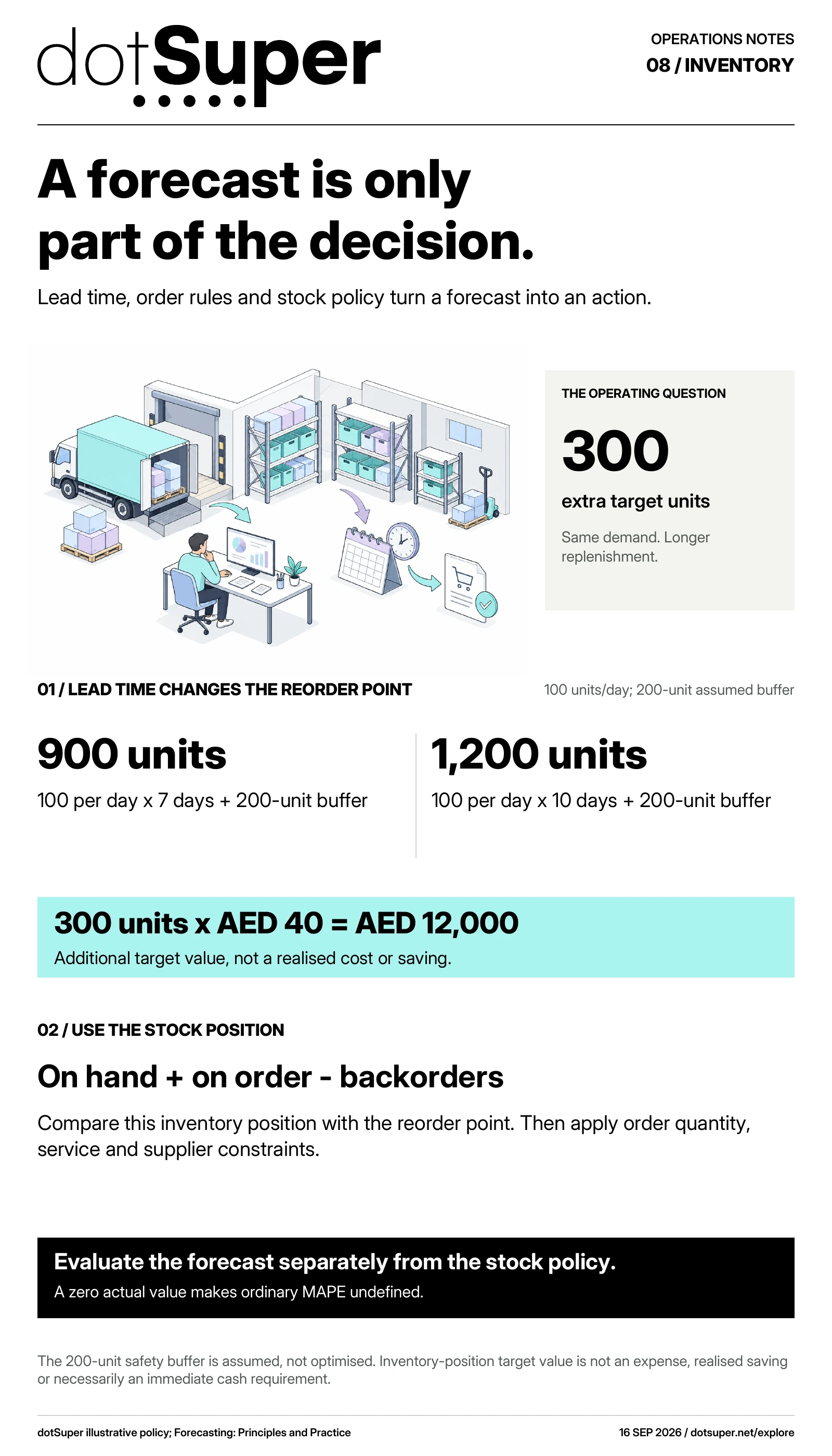
Reuse: Original artwork created for dotSuper. No public reuse licence has been specified. Attribution to research sources does not grant rights to their artwork or datasets.
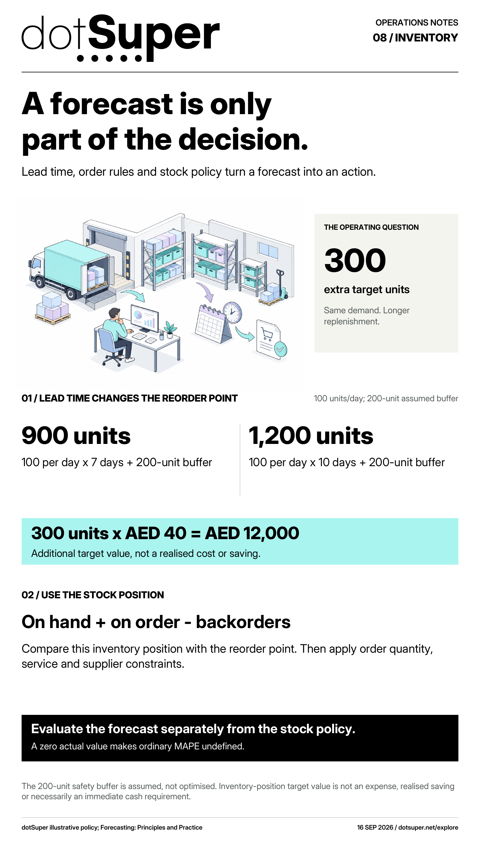
Read the diagram: Lead time, order rules and stock policy turn a forecast into an action. The 200-unit safety buffer is assumed, not optimised. Inventory-position target value is not an expense, realised saving or necessarily an immediate cash requirement.
With fictional demand of 100 units a day and a 200-unit buffer, a seven-day lead time gives a 900-unit reorder point. Ten days gives 1,200 units. The 300-unit change represents AED 12,000 at an assumed AED 40 per unit. Forecast accuracy still needs a separate evaluation.
At 100 units per day and an assumed 200-unit buffer, seven days of lead time gives 100 × 7 + 200 = 900 units. Ten days gives 1,200 units. The extra 300 units at an assumed AED 40 per unit have AED 12,000 of target value.
Inventory position is on-hand plus on-order minus backorders for the same item and location.
Two fictional observations: actual demand 0 and 20, forecasts 5 and 15. Both absolute errors are five. MAE is five units, MAPE undefined, and WAPE 10/20 = 50%.
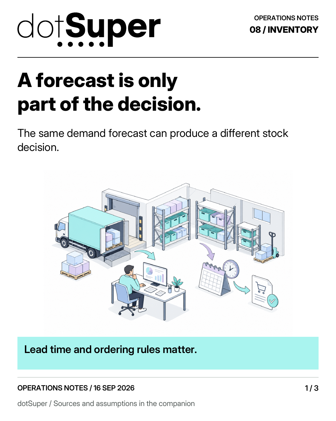
A forecast is only part of the decision. The same demand forecast can produce a different stock decision. Lead time and ordering rules matter.
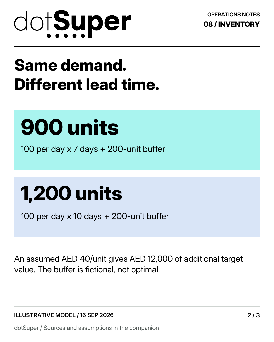
Same demand. Different lead time. 900 units / 100 per day x 7 days + 200-unit buffer 1,200 units / 100 per day x 10 days + 200-unit buffer An assumed AED 40/unit gives AED 12,000 of additional target value. The buffer is fictional, not optimal.
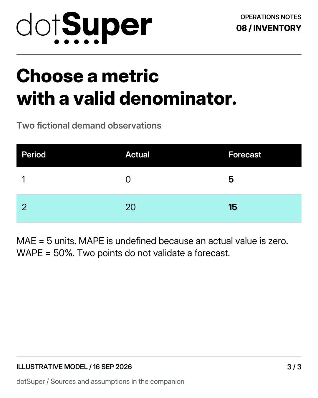
Choose a metric with a valid denominator. Two fictional demand observations 1 / 0 / 5 2 / 20 / 15 MAE = 5 units. MAPE is undefined because an actual value is zero. WAPE = 50%. Two points do not validate a forecast.
The 200-unit safety buffer is assumed, not optimised or tied to a proven service level.
Inventory-position target value is not necessarily an immediate cash requirement. On-order stock and payment timing matter.
Two observations illustrate metric arithmetic; they do not validate a forecasting model.
M5 evidence describes Walmart retail series, not regional firms, Gulf industrial demand or observed inventory outcomes.
| Dataset | Observation | Values and conditions |
|---|---|---|
| Fictional example: reorder scenarios | 7 | Demand/day: 100; Assumed buffer (units): 200; Reorder point (units): 900 |
| Fictional example: reorder scenarios | 10 | Demand/day: 100; Assumed buffer (units): 200; Reorder point (units): 1,200 |
| Fictional example: tiny accuracy example | 1 | Actual units: 0; Forecast units: 5; Absolute error: 5 |
| Fictional example: tiny accuracy example | 2 | Actual units: 20; Forecast units: 15; Absolute error: 5 |
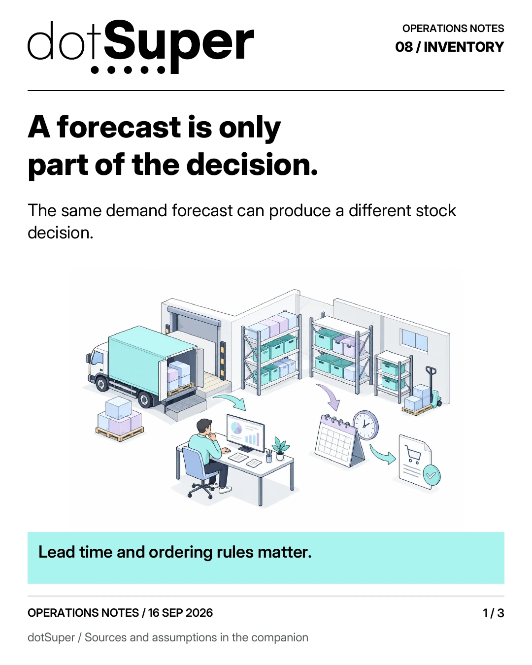
Reuse: Original artwork created for dotSuper. No public reuse licence has been specified. Attribution to research sources does not grant rights to their artwork or datasets.
Read the diagram: Panel 1 of 3. A forecast is only part of the decision.
A forecast is only part of the decision. The same demand forecast can produce a different stock decision. Lead time and ordering rules matter.
The 200-unit safety buffer is assumed, not optimised or tied to a proven service level.
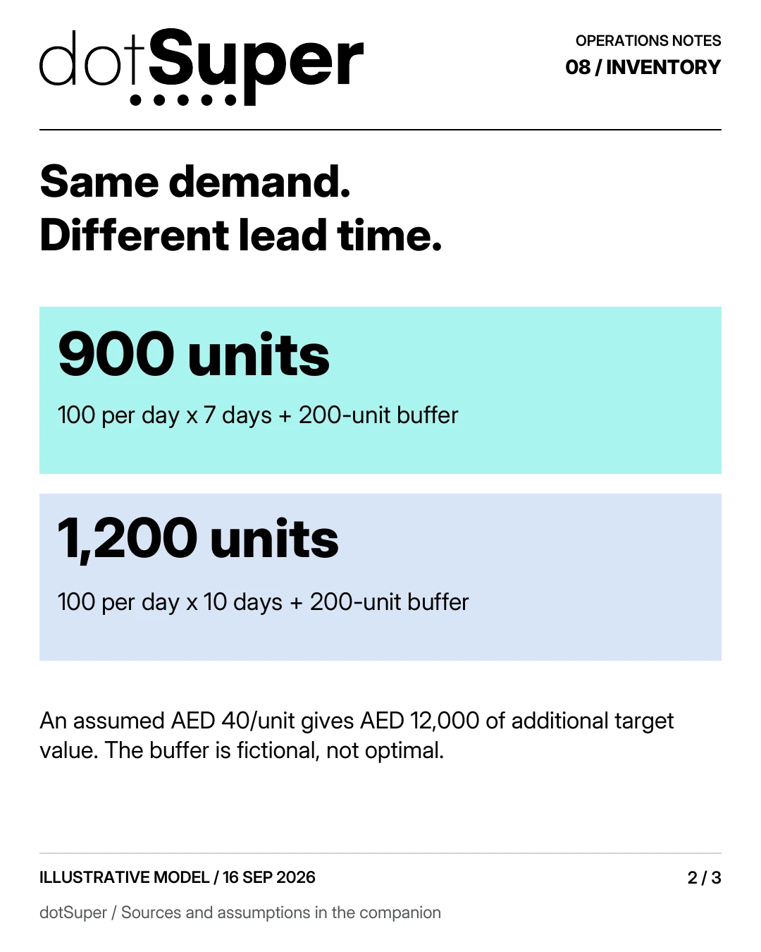
Reuse: Original artwork created for dotSuper. No public reuse licence has been specified. Attribution to research sources does not grant rights to their artwork or datasets.
Read the diagram: Panel 2 of 3. Same demand.
Same demand. Different lead time. 900 units / 100 per day x 7 days + 200-unit buffer 1,200 units / 100 per day x 10 days + 200-unit buffer An assumed AED 40/unit gives AED 12,000 of additional target value. The buffer is fictional, not optimal.
The 200-unit safety buffer is assumed, not optimised or tied to a proven service level.
Fictional example: reorder scenarios.
Lead time (days): 7; Demand/day: 100; Assumed buffer (units): 200; Reorder point (units): 900.
Lead time (days): 10; Demand/day: 100; Assumed buffer (units): 200; Reorder point (units): 1,200.
| Lead time (days) | Demand/day | Assumed buffer (units) | Reorder point (units) |
|---|---|---|---|
| 7 | 100 | 200 | 900 |
| 10 | 100 | 200 | 1,200 |
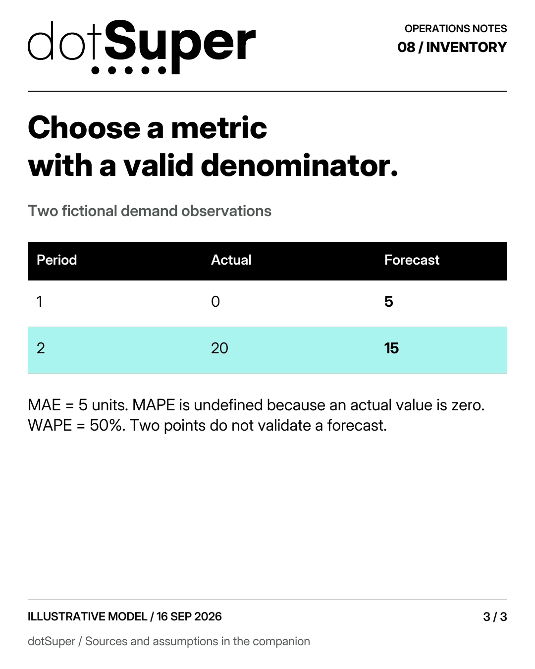
Reuse: Original artwork created for dotSuper. No public reuse licence has been specified. Attribution to research sources does not grant rights to their artwork or datasets.
Read the diagram: Panel 3 of 3. Choose a metric with a valid denominator.
Choose a metric with a valid denominator. Two fictional demand observations 1 / 0 / 5 2 / 20 / 15 MAE = 5 units. MAPE is undefined because an actual value is zero. WAPE = 50%. Two points do not validate a forecast.
The 200-unit safety buffer is assumed, not optimised or tied to a proven service level.
Fictional example: tiny accuracy example.
Observation: 1; Actual units: 0; Forecast units: 5; Absolute error: 5.
Observation: 2; Actual units: 20; Forecast units: 15; Absolute error: 5.
| Observation | Actual units | Forecast units | Absolute error |
|---|---|---|---|
| 1 | 0 | 5 | 5 |
| 2 | 20 | 15 | 5 |
Take it into your next working session
Keep the source credits with the file. Check the reuse terms and adapt the method to your context.
Credit: dotSuper original fictional worked-example data.
Reuse: Original illustrative data. No public reuse licence has been specified. These are not client measurements or research results.
Credit: dotSuper original fictional worked-example data.
Reuse: Original illustrative data. No public reuse licence has been specified. These are not client measurements or research results.
Reuse: Original artwork created for dotSuper. No public reuse licence has been specified. Attribution to research sources does not grant rights to their artwork or datasets.
Reuse: Original artwork created for dotSuper. No public reuse licence has been specified. Attribution to research sources does not grant rights to their artwork or datasets.
Reuse: Original artwork created for dotSuper. No public reuse licence has been specified. Attribution to research sources does not grant rights to their artwork or datasets.
Reuse: Original artwork created for dotSuper. No public reuse licence has been specified. Attribution to research sources does not grant rights to their artwork or datasets.
Reuse: Original artwork created for dotSuper. No public reuse licence has been specified. Attribution to research sources does not grant rights to their artwork or datasets.
Reuse: Original artwork created for dotSuper. No public reuse licence has been specified. Attribution to research sources does not grant rights to their artwork or datasets.
Thumbnail credit and reuse
Reuse: Original artwork created for dotSuper. No public reuse licence has been specified. Attribution to research sources does not grant rights to their artwork or datasets.
- 01At unchanged demand, a lead-time increase from seven to ten days raises the fictional reorder point from 900 to 1,200 units.
- 02The AED 12,000 difference is target inventory-position value, not expense or realised saving.
- 03MAPE is undefined in the two-observation example because one actual value is zero.
- 04Compare forecasts on unseen periods and inventory outcomes under an explicitly stated policy.
/ dotSuper point of view
A forecast matters through the replenishment decision it changes. Lead time, inventory policy and denominator choice can matter as much as the prediction model.
Audience, question and answer
Forecast the quantity and horizon needed for a real decision, compare against a simple baseline, and evaluate the inventory consequences.
A better average prediction does not automatically mean fewer stockouts or lower working capital.
Supplier lead times, minimum quantities, shelf life and service commitments determine what the forecast can change.
The scope includes operating businesses and manufacturers across markets.
Calendar effects, channels and replenishment routes need country-specific investigation.
Do not label every seasonal pattern “MENA demand” or assume a UAE distributor and a Saudi factory face the same replenishment conditions.
Research findings and their limits
It is substantial evidence that forecasting can be evaluated across a hierarchy, but it is retail competition evidence rather than a field trial at Gulf manufacturers.
Makridakis, Spiliotis and Assimakopoulos, M5 accuracy competition, International Journal of Forecasting 38(4), 2022 (source 4).
Hyndman and Athanasopoulos explain why evaluation should use genuinely unseen observations.
Their treatment also identifies problems with percentage errors when actual values are zero or near zero.
These problems matter for slow-moving spares and intermittent orders.
Forecasting: Principles and Practice, 3rd edition, section 5.8, live edition checked 16 September 2026 (source 1).
Rolling-origin evaluation moves the forecast origin forward while using only information available before each test period.
It can evaluate the horizon relevant to the purchasing decision rather than reward an easy one-day forecast.
Hyndman and Athanasopoulos, section 5.10, checked 16 September 2026 (source 3).
Prediction intervals make uncertainty explicit under the model's assumptions.
Their coverage still needs empirical checking.
An interval labelled 95% is not a guarantee that a particular delivery or demand realisation will lie within it.
Hyndman and Athanasopoulos, section 5.5, checked 16 September 2026 (source 2).
Begin with a decision contract
A buyer ordering weekly from a supplier with a four-week lead time needs a different horizon from a production supervisor allocating today's stock.
Use the inventory policy to define the required forecast, not the dashboard's default setting.
Distinguish demand from observed sales.
During stockouts, sales can understate what customers wanted.
A model trained without availability information can learn that a frequently unavailable item has low demand.
Record backorders, lost-order evidence where available, substitutions and promotions separately.
Do not manufacture an exact lost-demand series from unsupported assumptions.
Segment items by behaviour and consequence.
Fast movers, intermittent spares, new products, perishables and made-to-order materials have different problems.
Keep criticality separate from value: a cheap component can halt a valuable line.
The chosen service objective should reflect the business consequence of being short.
At the hierarchy level, reconcile forecasts with operational meaning.
A total forecast can be accurate while allocations across locations are wrong.
Moving stock between warehouses may be cheaper than buying more, but only if transfer lead time and permissions allow it.
The inventory action needs a location as well as an item.
What a fair pilot looks like
Freeze the historical information available at each forecast origin.
Do not let actual future promotions, revised orders or later supplier knowledge leak into a test that claims to simulate past decisions.
Test across relevant periods and item groups.
For Saudi and UAE operations, record local trading calendars and customer schedules as candidate predictors, then test whether they improve the defined horizon.
A calendar hypothesis is not evidence of a demand effect.
A short history may contain too few cycles to estimate that effect reliably.
Evaluate forecast error, bias and the inventory outcome under the same replenishment policy.
Then test the policy change separately.
Otherwise it is unclear whether improvement came from the model, different safety stock, more inventory or a changed service promise.
Log planner overrides and reasons before outcomes are known.
Some overrides add valuable local knowledge; others introduce bias.
Comparing override and non-override cases without considering why they were selected can be misleading.
Treat the analysis as diagnostic before making causal claims.
Worked example: the same forecast, a different lead time
An illustrative policy sets a 200-unit safety buffer.
The reorder point is 100 × 7 + 200 = 900 units of inventory position.
Inventory position here means on-hand plus on-order minus backorders, using the same item and location scope.
Suppose the supplier's lead time increases to ten days while expected daily demand remains unchanged.
The same assumed buffer produces a reorder point of 100 × 10 + 200 = 1,200 units.
The extra 300 units arise from lead time, not a higher demand forecast.
At an illustrative unit cost of AED 40, that difference represents AED 12,000 of additional inventory-position target value.
It does not mean AED 12,000 of expense or savings, and on-order stock may affect when cash moves.
The example does not establish an optimal safety buffer or a specified service level.
Now suppose minimum order quantity is 500 units and warehouse space is limited.
A 50-unit improvement in the point forecast may not change the next order at all.
A lead-time agreement or smaller order lot could have a larger practical effect.
That is a question to investigate, not an assumed result.
Quantitative context: avoid a misleading accuracy percentage
Absolute errors are five in each period, giving mean absolute error of five units.
Mean absolute percentage error is undefined because one actual value is zero.
Weighted absolute percentage error over this tiny example is 10/20 = 50%, but that aggregate hides the timing of overstock and shortage.
Do not publish the example as evidence that one metric is always best.
Select metrics based on the task, denominators and comparison groups.
An aggregate metric can give high-volume items most of the weight, obscuring a small but critical spare.
Always show the item count, period count and weighting rule.
For production reporting, include fill rate with its exact definition, stockout duration, inventory value, expedites, write-offs and forecast bias.
Distinguish order-line fill rate from unit fill rate and cycle service level.
Do not call them interchangeable “availability” percentages.
Evidence and boundaries
Each source supports only the scope stated beside the claim.
| Claim | Evidence | Limit |
|---|---|---|
| Forecast evaluation can span a hierarchy | M5 2022 paper | Walmart retail data, not Gulf manufacturing |
| In-sample fit is insufficient | FPP3 section 5.8 | General methodological guidance |
| Zero actuals can break MAPE | FPP3 section 5.8 | Choose alternatives appropriate to the task |
| Rolling origins preserve temporal ordering | FPP3 section 5.10 | Still vulnerable to incorrectly dated features |
| Prediction intervals depend on assumptions | FPP3 section 5.5 | Check actual coverage and drift |
| Lead-time change adds 300 target units | Fictional 100 × (10 − 7) | Buffer is assumed, not optimised |
| Example target-value difference is AED 12,000 | 300 × AED 40 | Working-capital context, not expense savings |
One practical next step
Compare the current process with a simple forecast baseline using only information available at each decision date.
Counterevidence and limitations
Sophisticated models can improve benchmark scores while leaving ordering decisions unchanged because of lot sizes or supplier constraints.
A forecast cannot create missing capacity, eliminate customs uncertainty or guarantee supplier performance.
Promotions, product introductions and structural changes can invalidate historic relationships.
A model trained on a past catalogue may fail on new items.
Preserve a fallback policy and a named planner who can explain an override.
That responsibility is part of the system, not evidence that the forecast has failed.
No local stockout, forecasting-adoption or inventory-turn benchmark is claimed.
The M5 numbers describe competition series, not firms or warehouses sampled across a region.
Search interest in inventory AI remains unmeasured.
What this page cannot conclude
- 01The 200-unit safety buffer is assumed, not optimised or tied to a proven service level.
- 02Inventory-position target value is not necessarily an immediate cash requirement. On-order stock and payment timing matter.
- 03Two observations illustrate metric arithmetic; they do not validate a forecasting model.
- 04M5 evidence describes Walmart retail series, not regional firms, Gulf industrial demand or observed inventory outcomes.
Sources
- 01Forecasting: Principles and Practice, 3rd edition, section 5.8, live edition checked 16 September 2026Hyndman and Athanasopoulos; OTexts · accessed Sep 16, 2026
- 02Hyndman and Athanasopoulos, section 5.5, checked 16 September 2026Hyndman and Athanasopoulos; OTexts · accessed Sep 16, 2026
- 03Forecasting: Principles and Practice, section 5.10Hyndman and Athanasopoulos; OTexts · accessed Sep 16, 2026
- 04Makridakis, Spiliotis and Assimakopoulos, M5 accuracy competition, International Journal of Forecasting 38(4), 2022Makridakis, Spiliotis and Assimakopoulos; International Journal of Forecasting · accessed Sep 16, 2026
Our editorial standard · Found an error? Send a correction with its source.
/ CITE OR SHARE THIS GUIDE
Make the evidence easy to verify.
When you reference this guide, link to its canonical URL. That gives readers one stable place for the evidence, limitations and future updates.
dotSuper Research Desk. (September 17, 2026). A forecast is only part of the decision.. dotSuper. https://dotsuper.net/feeds/applied-systems/forecasts-and-inventory-decisions